
How to Highlight Cells Rules with Conditional Formatting in Spreadsheets
How to Highlight Cells Rules with Conditional Formatting in Spreadsheets
Conditional formatting can easily spot trends and patterns in your data using bars, colors, and icons to visually highlight important values.
Highlight Cells Rules
To highlight cells that are greater than a value, follow the steps as below:
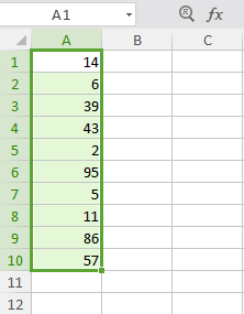
1. Select the range A1:A10.
2. Click the Conditional Formatting icon in the Home tab and choose Highlight Cells Rules in the drop-down list.
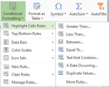
3. There are many options to choose, such as, Greater Than..., Less Than..., Between...(Here take the Greater Than... as an example). If you want to highlight cells that are greater than a value, choose Greater Than option and the Greater Than dialogue box will open, shown as below:
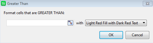
You can enter a value and select a formatting style. Here enter 75.
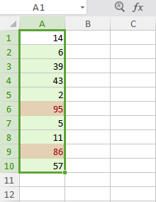
4. Click the OK button to complete this operation and the result as below:
5. If you change the value of cell A1 to 90, the result as below:
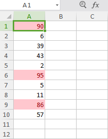
The Spreadsheets changes the format of cell A1 automatically.
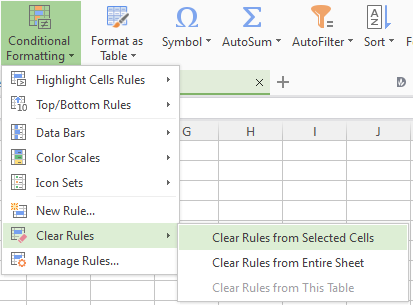
6. If you want to clear a conditional formatting rule, choose Clear Rules option in the drop down list. There are three options to choose: Clear Rules from Selected Cells, Clear Rules from Entire Sheet, and Clear Rules from This Table.
How to Highlight Cells Rules with Conditional Formatting in Spreadsheets
Conditional formatting can easily spot trends and patterns in your data using bars, colors, and icons to visually highlight important values.
Highlight Cells Rules
To highlight cells that are greater than a value, follow the steps as below:
1. Select the range A1:A10.

2. Click the Conditional Formatting icon in the Home tab and choose Highlight Cells Rules in the drop-down list.

3. There are many options to choose, such as, Greater Than..., Less Than..., Between...(Here take the Greater Than... as an example). If you want to highlight cells that are greater than a value, choose Greater Than option and the Greater Than dialogue box will open, shown as below:

You can enter a value and select a formatting style. Here enter 75.
4. Click the OK button to complete this operation and the result as below:

5. If you change the value of cell A1 to 90, the result as below:

The Spreadsheets changes the format of cell A1 automatically.
6. If you want to clear a conditional formatting rule, choose Clear Rules option in the drop down list. There are three options to choose: Clear Rules from Selected Cells, Clear Rules from Entire Sheet, and Clear Rules from This Table.

Not what you're looking for?
 Join our Facebook Group
 Feedback
