
How to Use AutoFilter Function in WPS Spreadsheets
Filter Data in a Table
Filters provide a quick way to find and work with a subset of data in a range or table. When you filter a list, you temporarily hide some of the data, so you can focus on the data you want.
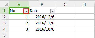
Step 1: Select a cell within the data that you want to filter.
Step 2: Click the AutoFilter icon in the Data tab and choose AutoFilter option in the drop-down list. Then a drop-down arrow will appear in the columns header.
Step 3: Click the drop-down arrow of the column you want to fliter.
Step 4: Choose the boxes of the items you want to show in the table.
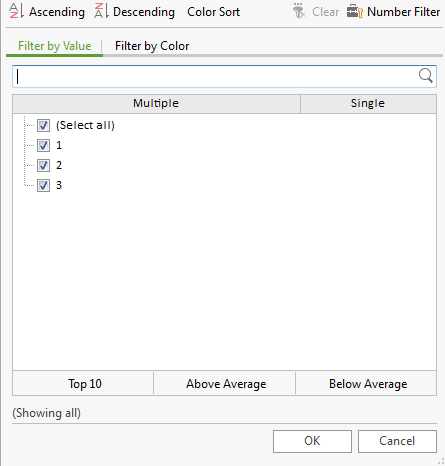
You can choose Ascending or Descending and "Filter by Value" or "Filter by Color" in the above dialogue box.
Step 5: Click the OK button to complete this operation. And the filtering arrow in the table header changes to this icon , which indicate a filter is applied.
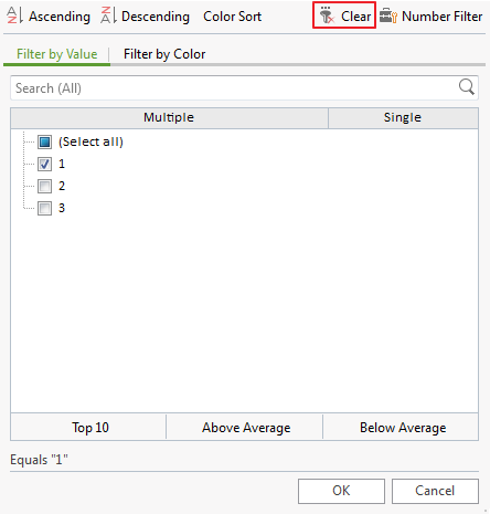
Note: If you want to clear filter, you can click the AtuoFilter icon again or choose the Clear icon in the above dialogue box, shown as below:
Filter Data in a Table
Filters provide a quick way to find and work with a subset of data in a range or table. When you filter a list, you temporarily hide some of the data, so you can focus on the data you want.
Step 1: Select a cell within the data that you want to filter.
Step 2: Click the AutoFilter icon in the Data tab and choose AutoFilter option in the drop-down list. Then a drop-down arrow will appear in the columns header.
Step 3: Click the drop-down arrow of the column you want to fliter.

Step 4: Choose the boxes of the items you want to show in the table.

You can choose Ascending or Descending and Filter by Value or Filter by Color in the above dialogue box.
Step 5: Click the OK button to complete this operation. And the filtering arrow in the table header changes to this icon , which indicate a filter is applied.
Note: If you want to clear filter, you can click the AtuoFilter icon again or choose the Clear icon in the above dialogue box, shown as below:

Not what you're looking for?
 Join our Facebook Group
 Feedback
