How to Freeze window in Spreadsheets 2016

Usually, we edit a large number of rows and columns in Spreadsheets. But when scrolling, it is inconvenient to keep the row or column label shown all the time. Sometimes we need to check the labels for the data in some rows or columns. We don’t want the row or column to move, for which it is very helpful to freeze the window.

The steps to freeze the window are shown as below:

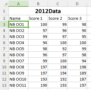
1. Select the leftmost cell of the cell range you want to freeze in the worksheet.

2. Click the Freeze icon in the View tab.

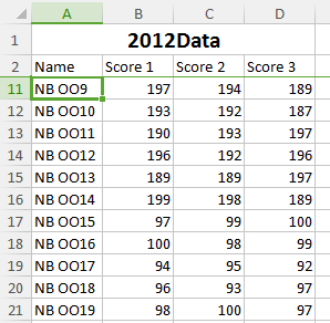
3. There will be a line above the selected cell range. Drag the scroll bar and the rows and columns in the frozen range won’t scroll. The frozen range is always in the top and left-most position. See below:

4. Click the Unfreeze icon in the View tab and you can cancel this operation.